Contents
History of physics in video games
Computational physics, computer graphics physics and real time physics
Modelling techniques
Computational physics, computer graphics physics and real time physics
Modelling techniques
- Pre-calculated animations
- Particle systems
- Rigid bodies
- Mass spring systems
- Finite Elements Method (FEM)
- Shallow Water Equations (SWE) method
History of physics in video games
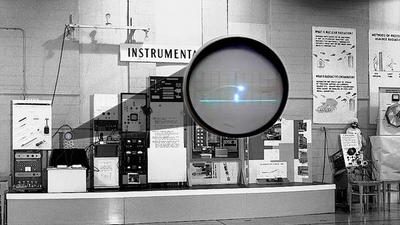
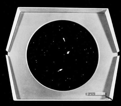
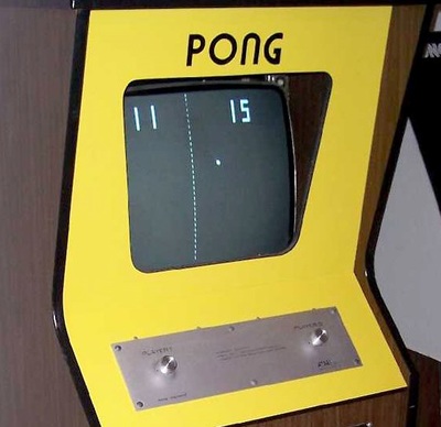
Physics modelling has been an important part of video games since their early days. The first game to incorporate physics was Tennis for Two (1958), which used ballistic equations to calculate the trajectory of a bouncing dot in the screen of an oscilloscope. Spacewar! (1962) incorporated the general gravity equation into its game play to simulate the gravitational pull of the central star on the screen. It was quite difficult to play, since it was difficult manage the gravitational pull of the star. The only physics used in the game that popularized video games, Pong (1972), was collision detection and response techniques to detect if the ball hit a paddle and how to bounce it back to the other player. After Pong, Donkey Kong (1981) revolutionized the known game play by adding jumping mechanics.

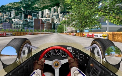
The vehicle simulation genre started to use physics with SubLogic Flight Simulator 1 for Apple II and TRS-80 (1980), which made use of rigid body dynamics to simulate the movement of the plane. But realistic car driving was not incorporated to video games until the late nineties, with games like Grand Prix Legends (1998). This was due to the added complexity of car physics, which had to model the response of the 4 wheels and the suspension to the steering wheel and the terrain among other issues.
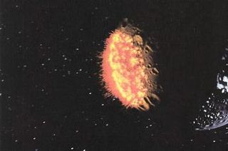
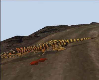
The first appearance of dynamic particle systems in computer graphics was in Star Trek II: The Wrath of Khan (1982), concretely to model the action of the Genesis device. Since then, particle systems are widely used in video games. Jurassic Prak: Trespasser (1998) was a milestone in physics for video games, since was the first one to incorporate inverse kinematics and ragdoll physics to move its characters.
Until the early 2000s, each game had its own physics modelling, so the game developers had to program all its physics. Physics engines changed this by externalizing the physics programming, and so allowing the development of more complex physics for video games. Many physics engines exist today, the video below shows the combination of Havok Physics from Havok, Euphoria from Natural Motion and DMM from Pixelux, used in Star Wars:The Force Unleashed.
Computational physics, computer graphics physics and real time physics.
Computational physics, physical simulations in computer graphics and real time physics are aimed to model our world, but they are focused into different aspects:
- Computational physics: Its aim is to understand and accurately model reality.
- Computer graphics physics: its aim is to reproduce the visual effects of physic processes.
- Real time physics: its aim is to allow the user to interact with the physics simulation.
The video below shows water flowing past a cylinder, modeled using the Computational Fluid Dynamics open source code OpenFOAM. The aim of this simulation is to be accurate, and its results are compared with experimental data at the end of the video.
The following video is a short animation I did using the software RealFlow, which does fluids and dynamics simulation for computer graphics. The equations in RealFlow follow the laws of physics, but what you see in the video is no exactly what it seems. First of all, the flame is modeled as a gas at a very low temperature (around 4Kelvin), so its particles don´t have enough energy to escape the volume where they are. Gravity is affecting the water but not the flame. Instead of it, an invisible object above the candle attracts the gas particles, so they form the shape of a flame. This makes clear that the aim of this simulation is not accuracy, it is visualization. Moreover, all the parameters and objects in this simulation are tuned to obtain the result shown in the video. This can be done because the simulation is not in real time, so it can be modified and repeated to obtain the desired result.
The third video is from the Batman GameWorkds video game, which uses the NVidia PhysX physics engine. As you can see, smoke reacts to the player's actions in real time.
Being able to perform this interaction comes with two challenges:
- Time: video games run at a fixed time rate of 30-60 Hertz (o fps). This leaves between 15 and 30 milliseconds to perform all calculations needed to generate each frame. These include game logic, AI, graphics and of course, physics.
- Stability: the physics simulation has to produce reasonable results in all imaginable situations within the game. If it fails to do so the game-play will be disrupted. It is difficult to take into account all imaginable situations, since they depend on the actions of the player. Some of them can go through development inadvertently, then is when physics glitches appear. The video at the right shows an example in the Read Dead Redemption video game developed by Rockstar games using the RAGE game engine. In it, the carts start oscillating without control for no apparent reason. I suspect the reason for this glitch is that the oscillatory movement of the cart enters resonance under some uncontrolled circumstances.
Modelling techniques
There is a great variety of techniques to model physics processes in video games. I will now introduce some of them.
Pre-calculated animations
This technique pre-calculates the movement of the object and saves and animation for it. When this action is required during the game, the animation is reproduced. No calculation is done in real time, so the animation will not interact with the player. Pre-calculated animation can also be combined with real time calculations to provide some interaction . Another example is to calculate part of the model and put the results in tables, then, in real time, look up for the convenient value for the current situation.
Particle systems
Particle systems are widely used in video games to model fuzzy objects, from spells and aesthetic animations to rain, smoke or water.
A particle system is a collection of many tiny objects called particles. Over time, particles are generated into a system, move and change from within the system and die from the system. Particles are represented as points, they have no physical shape, so they can't collide with each other.
Each particle has a set of attributes: position, velocity, mass and lifespan among many others depending on the model.

Particle system to model a galaxy
The diagram below shows the steps to model a particle system. For more information on particle systems here is a link to the article by William T. Reeves.

The following video is from a 3D scenario I programmed using OpenGL and C++. The rain is a particle system. Its particles are generated in random positions at the top of the domain, their dynamic attributes tell them to update their position by a fixed distance each frame and they are destroyed when they hit the ground after displaying an animation. The particles are rendered one by one.
SPH (Smoothed Particle Hydrodynamics) is an interpolation method for particle systems. This method is widely applied to model fluids with particles, though it was originally conceived fro astrophysics. SPH incorporates mathematical functions called kernels to the equations describing the movement of the particles. These functions allow to evaluate anywhere in space attributes that are only defined at discrete positions. For example, they allow to calculate the velocity of a particle taking into account the velocities of the particles surrounding it. To know more about SPH for fluids you can read the paper from Matthias Müller.
The next video shows water simulated using SPH. The model has 20million particles and it is not computed in real time. Instead of drawing the particles one by one like in the previous video, this one shows the envelope of the particle system, giving it the appearance of just one entity, water.
Rigid bodies
Rigid
bodies an important part of most game physics engines, since most
objects around us can be considered as non-deformable. Moreover, representing
objects as rigid bodies stores more physical information about each
object than particle systems but is still effective in terms of
simulation speed and memory footprint.
With particle systems, each object in the system is modeled as a single point with some attributes. Using rigid bodies, though, each object has also information about its physical shape and orientation. So objects can collide with each other, but they will not deform.
With particle systems, each object in the system is modeled as a single point with some attributes. Using rigid bodies, though, each object has also information about its physical shape and orientation. So objects can collide with each other, but they will not deform.
The attributes of each object are:
The diagram below explains the steps to model a rigid bodies system. For more information on rigid bodies in real time physics you can consult the notes of the course Real Time Physics by Matthias Müller, Jos Stam, Doug James and Nils Thürey; Chapter 6. Rigid Body Simulation.
- Position x of its center of mass.
- Orientation R. Represented by a rotation matrix or a quaternion.
- Linear velocity v at which the center of mass and the whole object moves.
- Angular velocity w of the object about its center of mass.
- Mass m of the object.
- Inertia tensor J of the object.
The diagram below explains the steps to model a rigid bodies system. For more information on rigid bodies in real time physics you can consult the notes of the course Real Time Physics by Matthias Müller, Jos Stam, Doug James and Nils Thürey; Chapter 6. Rigid Body Simulation.

The following video shows a rigid body simulation using the physics engine Bullet Physics.
Ragdolls are a subset of rigid body modelling. To create a ragdoll you have to build its skeleton by joining rigid bodies together.They are attached to each other by one of their extremes and are allowed to rotate and/or translate around the joints. The system is described by its degrees of freedom, which are the movements allowed at each joint. Moreover, the range of each movement can be restricted to suit the needs of the model. For example, a human forearm can rotate around the elbow to the shoulder and also along its length, so it has two degrees of freedom. Moreover, its movement is restricted to 180deg.

Rigid body skeleton with the movements allowed at each joint.
|
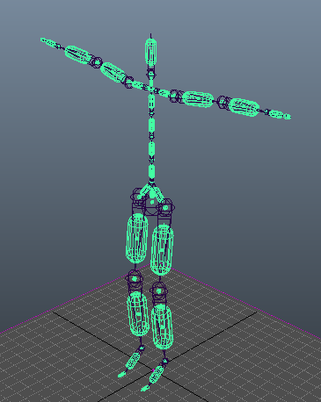
Skeleton for a ragdoll in Maya. The physics engine Bullet physics will compute its movement
|
Ragdolls are mainly used to model bodies falling to the ground. The next video shows ragdoll physics in Skyrim.
They can also be used to move a character from one position to another. For example to blend the end of one animation with the beginning of the next one or to make the character pick an object. In these cases we know the initial and final state of the ragdoll and we need to calculate the intermediate states, this is modeled using Inverse Kinematics (IK).
The following videos show two animations of a robotic arm I modeled as an exercise for the computational physics course. The system has 9 joints and 9 degrees of freedom, since each joint is only allowed to rotate about one axis. The aim of the exercise was to calculate the intermediate states of the arm that will move its end 4m along the floor. The video in the left shows the animation with no restrictions in the joints movement, while in the one on the right the 5th joint was not allowed to change its angle. I calculated the state of the arm at each frame using Inverse Kinematics with the pseudo inverse Jacobian method. I programmed the model with Fortran and rendered it with Pov-Ray.
|
|
|
The Euphoria engine by Natural Motion combines ragdolls and inverse kinematics with Artificial Intelligence to model characters that move in a physically correct way and react to their environment.
Mass spring systems
Video games use the mass-spring method to model deformable bodies like rubbery objects, cloth, hair or even cars.
The mass spring method allows to model deformable solids. With it, each object in the system is modeled as a set of point masses connected by strings. It is easy to program and fast but has some drawbacks:
Each object in the system is composed by a set of N particles with masses mi, positions xi and velocities vi. These particles are connected by a set of S springs with rest length l0, stiffness ks and damping coefficient kd. The distribution of the masses and strings can be taken from the graphical mesh used to draw the object, although it is recommended not to use exactly the same one, since it can have characteristics not suitable for physics modelling like duplicated vertices or intersecting triangles.
The diagram below explains the steps to model a system of objects using the mass spring method. For more information I leave a link to the notes of the course Real Time Physics by Matthias Müller, Jos Stam, Doug James and Nils Thürey; Chapter 3. Mass spring systems.
The mass spring method allows to model deformable solids. With it, each object in the system is modeled as a set of point masses connected by strings. It is easy to program and fast but has some drawbacks:
- The behavior of the object depends on how the spring network is set up.
- It can be difficult to adjust the string constants to obtain the desired behavior.
- Mass spring systems model an object as a collection of points and strings, it does not take into account the volume between the strings. So it can't capture volumetric effects, for example it can't assure that the objects maintain their volume.
Each object in the system is composed by a set of N particles with masses mi, positions xi and velocities vi. These particles are connected by a set of S springs with rest length l0, stiffness ks and damping coefficient kd. The distribution of the masses and strings can be taken from the graphical mesh used to draw the object, although it is recommended not to use exactly the same one, since it can have characteristics not suitable for physics modelling like duplicated vertices or intersecting triangles.
The diagram below explains the steps to model a system of objects using the mass spring method. For more information I leave a link to the notes of the course Real Time Physics by Matthias Müller, Jos Stam, Doug James and Nils Thürey; Chapter 3. Mass spring systems.

This video from World of Goo, which uses the Open Dynamics Engine physics engine, shows mass spring systems at work.
The following video is from the vehicle simulator BeamNG.drive, which uses the mass spring method to model the cars.
Finite Element Method (FEM)
The Finite Element Method treats each object in the system as a continuous volume. By doing so it overcomes the drawbacks of the mass spring systems but it is also more computationally expensive. We use FEM to model deformable objects when the precision offered by mass spring systems is not enough and/or its drawback become important. For example, FEM allows you to assign a material to an object to determine how it bends and breaks. This is not possible with the mass-spring method, since you can only modify the particles and springs that form an object, not the object as a whole.
For more information on Finite Element Method in real time physics you can consult the notes of the course Real Time Physics by Matthias Müller, Jos Stam, Doug James and Nils Thürey; Chapter 4. The Finite Element Method.
The physics engine Digital Molecular Matter (DMM) from Pixelux uses FEM to model the deformation and fracture of solid objects. The next video shows DMM in Star Wars: The Force Unleashed.
Shallow Water Equations (SWE) method
The shallow Water equations model the water surface for shallow water flow as a river or a swimming pool. This method is faster than using the complete form of equations commonly used to model fluids but has some drawbacks:
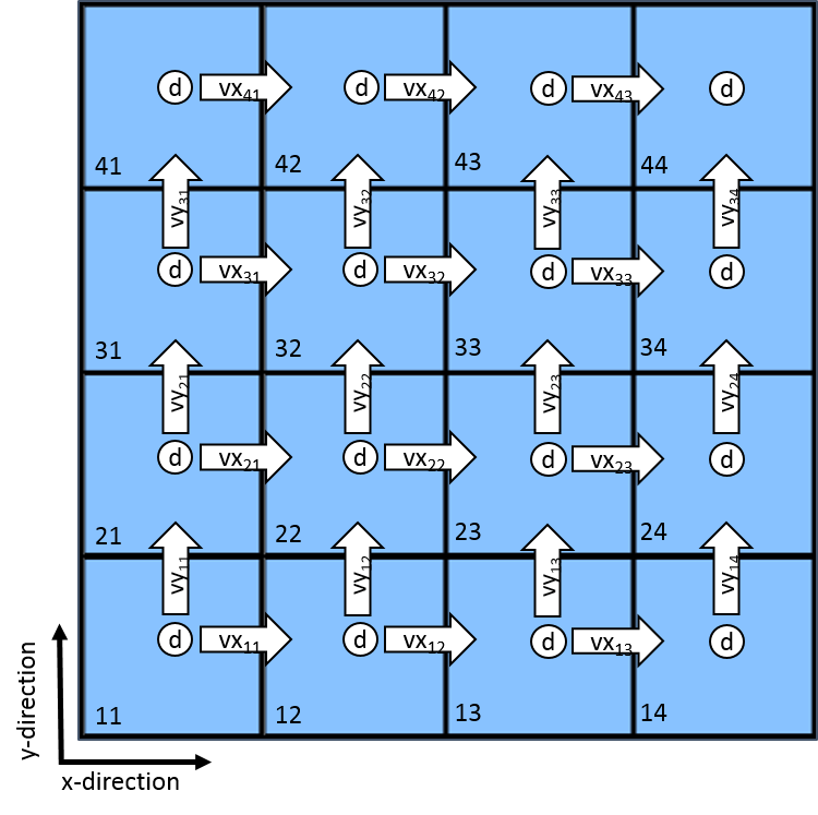
The water surface is divided into nx cells in x-direction and ny cells in y-direction. The attributes modeled at each cell are:
- It is unable to bend the surface of the water over itself. So it can´t model breaking waves, jets...
- It can only be applied to shallow water. It can´t model 3D flows as smoke in air or the mixing of two fluids.
The water surface is divided into nx cells in x-direction and ny cells in y-direction. The attributes modeled at each cell are:
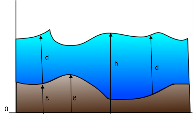
- The height h of water
- The height g of the ground
- The height d of water above the ground (d=h-g)
- The velocity vx of the water along the x-direction
- The velocity vy of the water along the y-direction
|
|
The first step to model the surface of the water is to initialize the attributes of the fluid in all its cells. Then, between each step of the motion:
The values at each cell depend on the values at its neighboring cells, but the cells on the boundaries are not surrounded by neighbors, so the characteristics of the flow there have to be specified. These are the Boundary Conditions. The left video shows an example where the boundary conditions are set to reflect the water that reaches the boundaries, while in the right video they are set to absorb the water that reaches them.
- Update attributes of the water at each cell. Unlike in the previous methods, here the modeled object does not move, is the water in its cells that changes. This method updates the height and velocity of the fluid in each cell using the Shallow Water Equations, which take into account the acceleration of the gravity and the amount of water that enters a cell from its neighboring cells.
- Use the height of water at each cell to draw the the water surface.
The values at each cell depend on the values at its neighboring cells, but the cells on the boundaries are not surrounded by neighbors, so the characteristics of the flow there have to be specified. These are the Boundary Conditions. The left video shows an example where the boundary conditions are set to reflect the water that reaches the boundaries, while in the right video they are set to absorb the water that reaches them.
|
|
|
For more information on the Shallow Water Equations in real time physics you can consult the notes of the course Real Time Physics by Matthias Müller, Jos Stam, Doug James and Nils Thürey; Chapter 11. Shallow Water Equations.
Physics engines use the shallow equations method to model flow over terrain as in the following video.
